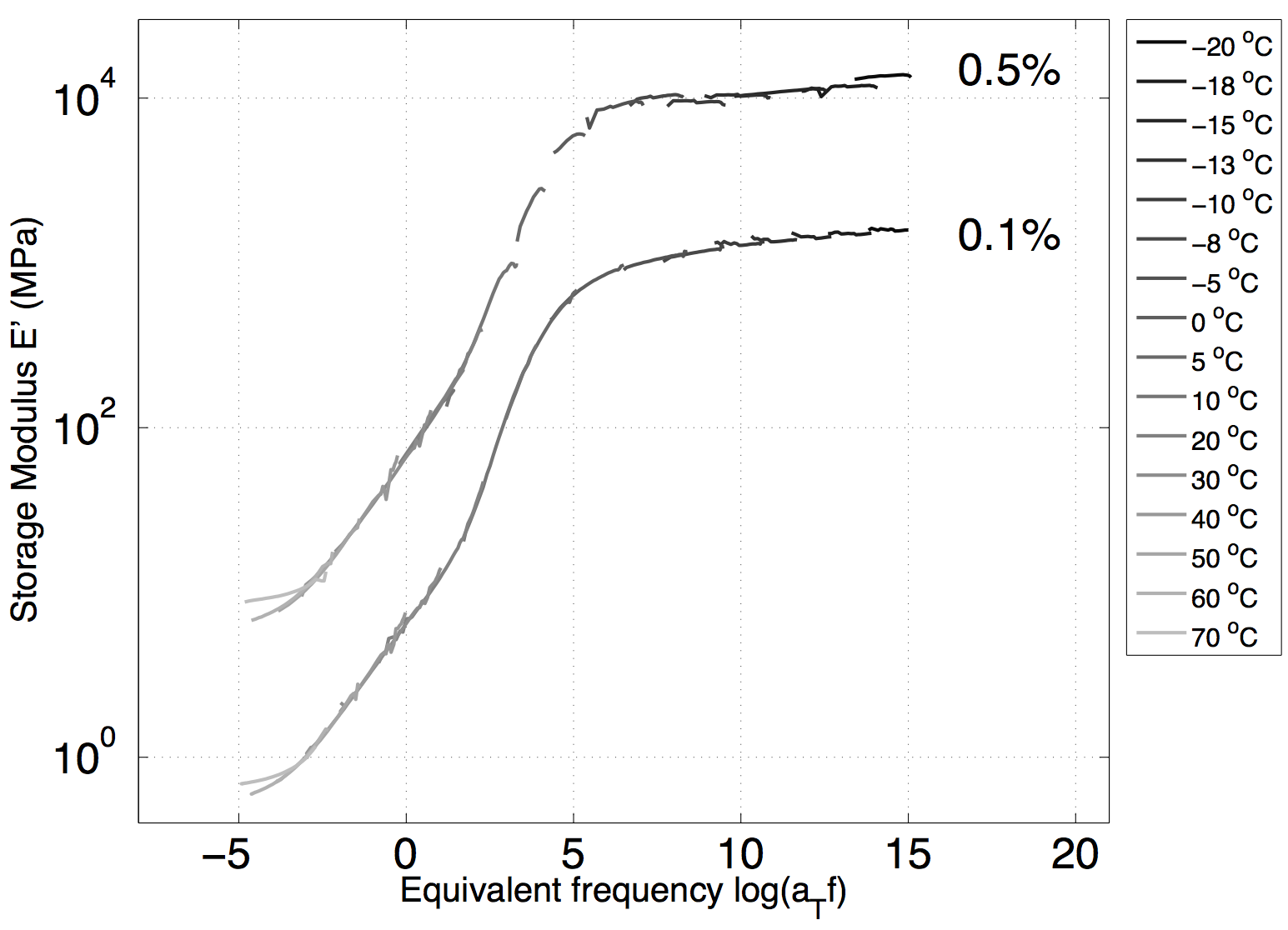
To build a mastercurve for any polymer means performing multiple tests spanning a wide range of frequencies and temperatures from below the glass transition to as high as possible but below the melting point. There are two ways of doing that, either scan multiple frequencies at each temperature (generally the fastest) or scan multiple temperatures at each frequencies.

The only way for LCEs is to program a test scanning a large number of frequencies at a unique temperature and repeat the process for each desired temperature. This is due to the fact that LCEs exhibit large changes in length according to temperature. As the strain control of the DMA is less performant than the displacement control, the new length has to be measured at each temperature in order to perform all the DMA tests at constant strain amplitude.

Step 1 Specimen preparation

Cut a rectangular specimen or the central part of a dumbbell specimen and measure its section.

Place the specimen in the DMA, measure the length. Be aware of the fact that the length will increase at low temperature so make sure that the length is small to stay within the limits of the machine (24 mm) at its maximum length.

CAREFUL do not tighten the grips too much or the specimen will break in the grips with the shape changes associated with temperature variation. On the other hand do not let them too loose or the specimen will slip out of the grips during the test. It might take several time to get a sense of how much is too much…

Make sure to record in your lab notebook all the dimensions (length, width, thickness) to get the volume at room temperature. Since the material is incompressible, it will allow you to compute the section at each temperature according to the measured length.

Step 2 Length measurement Perform a DMA test where

• the temperature equilibrates and holds at the chosen value
• the length is then measured at 0 force.

Record the length of the specimen at equilibrium.

Compute the corresponding strain amplitude for the DMA test, for example 0.1% of that length

Leave the specimen in the DMA

Step 3 DMA test

Input the length and the displacement amplitude in the software.

If wanted, compute the new section assuming incompressibility and input the new dimensions. If it is not done, it will just affect the computation of the moduli. However, these values can be computed afterwards using the raw data of the test.

Perform a DMA test where

• the temperature is equilibrated and held at the chosen value. You can use a time hold to make sure the temperature is stable before starting the mechanical test.
• scan the frequencies and measure the DMA properties. For LCEs, it appears that the low frequencies (lower than 50Hz) allow to build a clean mastercurve. The values measured at frequencies between 50 Hz and 70 Hz seem highly scattered while the material exhibit a highly nonlinear behavior at higher frequencies (above 70Hz).
• CAREFUL sometimes the DMA test does not start, generally due to the fact that these LCEs are extremely soft and the machine is having trouble regulating its displacement according to the low load response. One solution is to increase the preload. However, do not increase it too much otherwise you will significantly stretch the specimen before all measurements.

For each test, open the result file in the Universal Analysis software and export all the raw data as text files. Make sure to name your data files in a consistent manner to facilitate the post processing in Matlab.

The steps 2 and 3 are repeated for each temperature, generally something like every 5 or 10 degrees between -20C and 80C.

<fc #4682b4>For LCEs, only the glassy or nematic domains obey the time-temperature superposition, a mastercurve cannot be built through the nematic-isotropic transition.</fc>

As a consequence there is no point in measuring all temperatures above about 85C. Perform one test at 120C to get the isotropic behavior but it is not possible to build even a separate mastercurve of the isotropic phase.

For the example below, we used -20, -18, -15, -13, -10, -8, -5, 0, 5, 10, 20, 30, 40, 50, 60, and 70C. The curve at 80C did not fit on the mastercurve. The temperatures you need to get a smooth continuous mastercurve also depend on the amplitude.

Step 4 Matlab postprocessing

The function to read the raw data in Matlab is available on this wiki in the section Experimental Protocols subsection data analysis. The DMA function can be used to read all text files of raw data from the DMA.

Make sure to check that the storage modulus and loss modulus are computed from the stiffness and the dimensions of the specimens. The values produced by the DMA are potentially incorrect because of the section variation with temperature.

Open the results in Matlab and plot the storage modulus according to frequency in a loglog plot.

Shift horizontally each curve until the beginning of one curve overlaps the end of the neighboring curve using a shift factor a(T) (check the time temperature superposition theory in any book on Polymer viscoelasticity if you are lost).

<fc #4682b4>Once all the curves are shifted, you have a mastercurve!</fc>

If you have holes in between curves, that means you need more temperatures. In our example, although the chosen temperatures produced a smooth and nice curve at 0.1% amplitude, it was not the case when the amplitude was increased to 0.5%.